# ML – Support Vector Machines (SVM)

Linear SVM

The loss function for a logistic regression model is given by

$L = - [ \hat{y}\log{y} + (1-\hat{y})\log{(1-y)} ]$

The output of the logistic regression is defined as

$y = \frac{1}{(1 + e^{w^Tx})}$

Ideally, the weights should be as low as possible. To do so, we employ L2 regulrization. This also has a side effect of weight decay where the weights for non-contributing features tends to zero.

$L = -[\hat{y}\log{y} + (1-\hat{y})\log{(1-y)}] + \frac{\lambda}{2} ||w||^2$

where $\lambda$ is a regularization parameter.

The functions log(y) and log(1 - y) can be replaced by approximated cost functions.

$L = y\cdot cost_1(w^Tx) + (1 - y) \cdot cost_0(w^Tx) + \frac{\lambda}{2} ||w||^2$

Now, divide L by $\lambda$ .

$L = \frac{1}{\lambda}(y \cdot cost_1(w^Tx) + (1 - y) \cdot cost_0(w^Tx)) + \frac{1}{2} ||w||^2$

Let $\frac{1}{\lambda} = c$ . Then

$L = c(y \cdot cost_1(w^Tx) + (1 - y) \cdot cost_0(w^Tx)) + \frac{1}{2} ||w||^2$

This is equivalent to maximizing the margin which is given by $\frac{1}{||w||}$ between hyperplane and the data points in both classes.

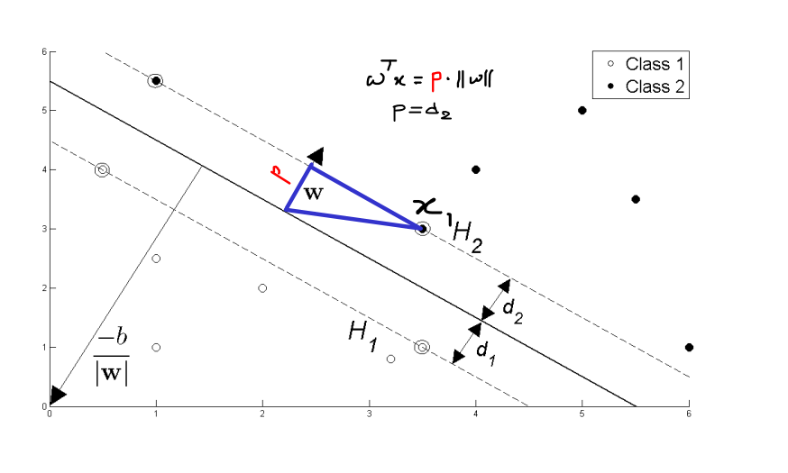
Here is how – Ideally,

$w^Tx_1 = 1$

But this can be written as (from projection theorem)

$d2 \cdot ||w|| = 1$

$d2 = \frac{1}{||w||}$

The aim of SVM is to maximize the distance between i.e maximize d2. Hence it is equivalent to minimizing ||w||.

Kernel Trick

Instead of just $w^Tx$ , one can use $f(w^Tx)$ . Generally, $f$ will be gaussian function and hence the input closer to Support Vectors gets activated and you try to minimize the cost function involving the kernels. The gaussian kernels are also called as Radial Basis Functions(RBF) because of the shape of the activation.

Extra Notes

The vector c is also called as lagrage multiplier. It is used to find the support vectors that maximizes the margin.

For complete explanation, refer to this link.

ML/DL Page

# ML – Support Vector Machines (SVM)

Linear SVM

Kernel Trick

Extra Notes

Leave a Reply Cancel reply